Saying that marketers are data-centric people is an understatement: Between return on investment, cost per acquisition and more, they’re always looking at different metrics and reporting on progress.
It can be tricky to keep all of those numbers straight, though. That’s where spreadsheets come in handy. With a well-organized spreadsheet, marketers can quickly analyze robust data sets and make smarter, more informed decisions about their efforts.
Originally introduced by Microsoft in 1987, Excel was the go-to tool for years for building spreadsheets. But when collaborative, cloud-based tool Google Sheets was introduced in 2012, many users made the switch over to this new (free!) resource.
If you’re also looking to get started with Google Sheets, you’re in the right place. In this guide, we’ll be looking at the benefits of Google Sheets and walking you through some of the basics so you can get up to speed quickly and efficiently.
The Benefits of Using Google Sheets for Marketing
First things first: Let’s talk about the benefits of using Google Sheets for marketing purposes before we discuss more traditional options (like a standard Excel spreadsheet).
- It’s cloud-based. Cloud-based spreadsheets are automatically saved, stored, and maintained via a remote server. That means that you can access it online from anywhere, any time. Plus: Google Sheets is also available offline.
- It’s free. No expensive software required — Google Sheets is always 100% free.
- It works across devices. Modern marketers switch between devices throughout the day — and Google Sheets accommodates that behavior. You can access and edit Google Sheet data from a wide variety of devices (like your smartphone, tablet, and computer).
- Add-ons are available. We’ll get into the specifics of add-ons for Google Sheets a bit later, but the increased functionality and flexibility of these additional features makes this spreadsheet tool even more versatile and powerful.
You might be wondering: What’s the difference between Google Sheets and Excel? The short answer is: price, collaboration, and flexibility.
While Excel requires a software subscription (which costs about $130), Google Sheets is free for all Google account holders. In terms of collaboration, Excel requires you to save and send a new version when edits are made, while Google Sheets automatically updates a single shared file for all team members. And lastly, because Google Sheets has the ability to accommodate many different integrations, it’s often more flexible than a standalone software solution like Excel.
Common Google Sheets Terms to Know
Next, let’s get familiar with some of the language and common terms used when referencing data within Google Sheets.
- Column: Columns are vertical cell sets.
- Row: Rows are horizontal cell sets.
- Cell: Cells are the single data points within a Google Sheet.
- Range: Range refers to a selection of cells across a column, row, or both.
- Function: Function refers to built-in operations for the Google Sheet that can be used to quickly calculate values, to manipulate data, and more.
- Formula: Formulas combine functions, rows, cells, columns, and ranges to generate a particular end result.
How to Use Google Sheets
Now we’re ready to dive into the more advanced how-to’s and lessons on using Google Sheets.
Understanding the Google Sheets Toolbar
One of the very first things to do is master the icons located in the Google Sheets toolbar. Doing so will help ensure you’re getting the most out of its abilities and that you’re saving time with shortcuts. Take a look at the screenshot below to identify some of the basic icons and their purposes within the toolbar.
How to Create a New Spreadsheet
When you’re ready to create a new spreadsheet, you’ll just need to follow a few quick steps to get started. Open Google Sheets and click "File" > "New" > "Spreadsheet".
Once you create your new spreadsheet, you can start adding data. If you want to work with an existing spreadsheet from Excel instead, you’ll need to import that data into your new Google Sheet.
How to Convert Excel to Google Sheets
When you need to import an Excel spreadsheet into Google Sheets, go to "File" > "Import" > "Upload" and then select a file that’s in one of the non-password protected formats (such as .xls, .csv, or .txt for example).
From there, your file will be uploaded and automatically converted into a Google Sheet.
Sharing and Protecting Your Data
Once your Google Sheet is set up and populated, you’ll want to think about how to share and protect your data. Data is automatically saved, so you don’t need to worry about that part. You can select who you share your file with and whether they have edit, comment, or view permissions. You can also protect specific data within your sheet so that those who have access can only edit certain cells.
To share a file:
- Go to "File" > "Share" (or just click the blue Share button in the top right corner)
- Enter the email address of who you’ll be sharing the spreadsheet with
- Assign permission levels (such as "View only" or "Can edit")
- Click "Advanced" and select any additional privacy conditions needed
To protect data:
- Navigate to “Data” > “Protected Sheets and Ranges”
- Choose “Range” or “Sheet” (to protect an entire sheet)
- Select the data you’d like to protect
- Click “Set Permissions”
- Choose to show an error warning to anyone who attempts to edit or customize editing permissions for certain people.
Organizing Data in Google Sheets
Google Sheets is a powerful tool that can hold a ton of data. That means the more data you have, the harder it becomes to find it — that’s when filtering comes in handy. Google Sheets has several filters that allow you to select the data you want to see and hide what you don’t.
How to Hide Data
Google allows you to hide entire rows or columns. This becomes useful when you want to restrict views for sharing, or when you’d like to control the amount of data you’re viewing at any given time. To hide a column, right-click the column you want to hide, then select “Hide Column”. When you hide a column, two arrows will appear on the previous and subsequent columns. Click these to restore the column to full view.=
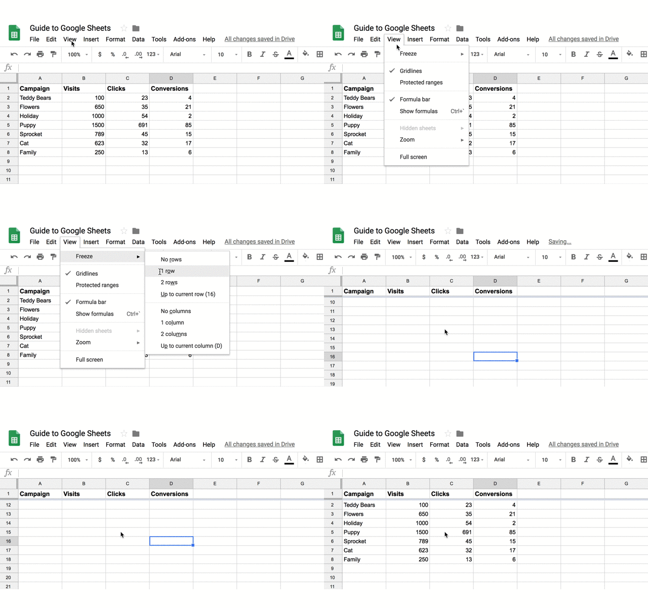
How to Freeze Rows and Columns
Freezing will create a floating row or column as you scroll and keeps the data in those fields within your line of sight. For example, if you use the first row to label your columns, you can freeze that row so you don’t have to remember what each column is as you scroll.
To freeze a row, select “View” > “Freeze” > “1 row” (or up to X rows).

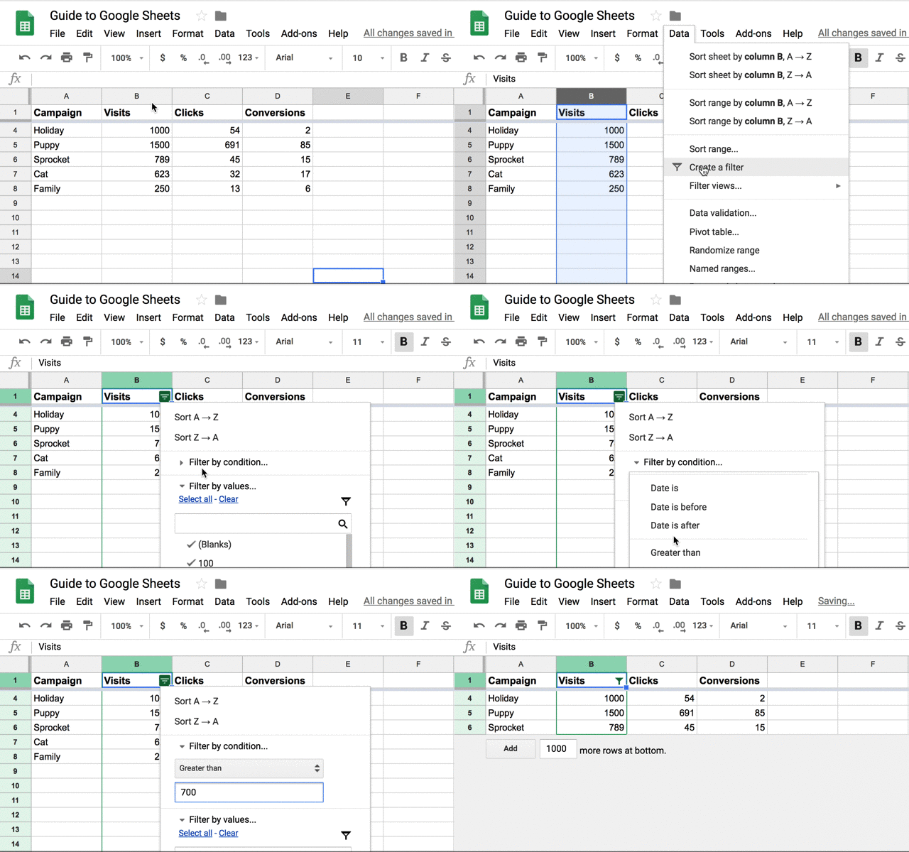
How to Filter Data
What if you’d like to view all of the data in a single column that fits a certain criteria? Apply a filter. Filters allow you to select a criteria and how that criteria applies to your data. For example, you can filter your ‘Site Visits’ column to show all values greater than 1000, or filter your sheet for all cells that have the word “cat”.
To set up a filter, select “Data” > “Create a Filter.” Click the funnel icon that appears in the column, then choose to filter by condition, value, or alpha or numeric order. Your sheet will only display data that satisfies your criteria.
Learn about other filtering options below.
How to Setup and Use Google Sheets Offline
If you need to use Google Sheets offline, just follow the steps outlined here to turn on offline access to your spreadsheets.
Keep in mind:
- You must be connected to the internet.
- You'll need to use the Google Chrome browser (don't use incognito mode)
- You'll need to install and enable the Google Docs Offline Chrome extension.
- Make sure you have enough free space on your device to save all your files.
From there:
- Open Chrome and make sure you're signed in.
- Go to drive.google.com/drive/settings.
- Check the box next to "Sync Google Docs, Sheets, Slides & Drawings files to this computer so that you can edit offline."
- To work on files offline from a computer, learn how to install Backup and Sync.
Advanced Google Sheets Tips
Now that you understand the basics of Google Sheets, let’s get into some advanced tips so you can start using Sheets like a pro. These tips are helpful to have in your back pocket … even if you don’t need them just yet.
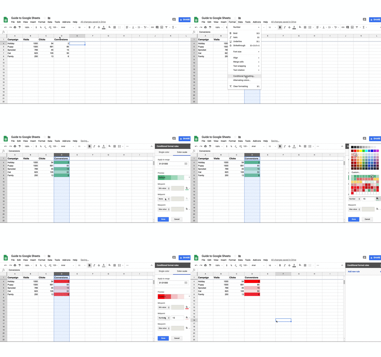
Conditional Formatting and Heatmaps
Conditional formatting will automatically apply formatting to a cell based on a preset condition. For example, you can select to highlight a cell in red if the value entered is below 100 or reads “Error”.
Heatmaps work similarly in that they apply a color scale to cells based on a median criteria (values greater than the median will appear darker while values lesser will appear lighter). This helps you view values on a gradient and identifies areas of concern on which to focus your attention.

Array Formulas
Array formulas can perform multiple calculations at once and output a value based on those calculations. Whereas most formulas require you to perform each step independently (e.g. sum one row then add it to the sum of the subsequent row), arrays make calculations much more efficient. This helps when working with large amounts of data.
Macros
The Macros feature records a series of steps that you’d like Google Sheets to repeat on command. For instance, if you work with a new data set each month, and need to manipulate that data in the same sequence each time, then you can record a Macro, and have Google do the work for you.
10 Must-Know Google Sheets Formulas
When you've entered your data and you need to do some quick number-crunching, basic formulas can help you find the answers you need. Here are a few commonly used Google Sheets formulas to speed up your data analysis.
1. SUMThis formula adds all values within a selected range.
=SUM(range)
2. AVERAGEThis formula calculates the average of values within a range.
=AVERAGE(range)
3. FILTERThis formula returns a filtered version of the source range, returning only rows or columns which meet the specified conditions. This is helpful when segmenting data by year or month.
FILTER(range, condition1, [condition2])
4. FINDThis formula returns the position at which a string is first found within the text. The Find formula is case sensitive.
FIND(search_for, text_to_search, [starting_at])
5. COUNTIFThis formula returns a conditional count across a range.
=COUNTIF(range, criterion)
6. CONCATENATEThis formula allows you to combine values of multiple cells into one cell, e.g., first and last name.
=CONCATENATE(Value1, “ ”,Value2)
7. VLOOKUPThis stands for vertical lookup. This formula searches down the first column of a range for a key and returns the value of a specific cell in the row found.
=VLOOKUP(search_key, range, index, [is_sorted]).
Learn how to do a VLOOKUP in less than a minute.
8. SPLITThis formula divides text around a specified character or string, and puts each fragment into a separate cell in the row. Use this when you want to break up first names from last names in a list of customers or prospects.
=SPLIT(text, delimiter, [split_by_each])
9. SUBSTITUTEThis formula replaces existing text with new text in a string. For example: You could replace a product name with a new one in a sheet of ad copy.
=SUBSTITUTE(text_to_search, search_for, replace_with, [occurrence_number])
10. PROPERThis formula edits text within a cell to title case so you don’t have to format each entry manually.
=PROPER (text)
For more formulas you can use in Google Sheets, use the search tool on the spreadsheet functions list and find the one you need.
Google Sheets Functions & Skills You Should Know
How to Create a Pivot Table
- Select the cells with source data you want to use in your pivot table. Note: Each column will need a header.
- In the menu at the top, click “Data” > “Pivot table.” Click the pivot table sheet (if it's not already open).
- In the side panel, next to "Rows" or "Columns," click "Add" and then choose a value. Note: Sometimes you will see recommended pivot tables based on the data you've selected. To add a pivot table, under "Suggested," select a pivot table.
- In the side panel, next to "Values," click "Add", then choose the value you want to see over your rows or columns. You can change how your data is listed, sorted, summarized, or filtered.
- Next to what you want to change, click the down arrow.
How to Remove Duplicates
- Select the cell in which you'd like to remove the duplicated info.
- Enter the function =UNIQUE(
- Select the cells you would like to pull data from
- Close the parentheses. Your function should look something like this: =UNIQUE(A:A)
How to Create a Drop-Down List
- Next to "Criteria," choose an option:
- Click "Data" > "Data validation".
- Select the cell or cells in which you want to create a drop-down list. List from a range: Choose the cells that will be included in the list.
- List of items: Enter items, separated by commas and no spaces.
- The cells will have a down arrow. To remove the arrow, uncheck "Display in-cell button to show list".
- If you enter data in a cell that doesn't match an item on the list, you'll see a warning. If you want people to only enter items from the list, choose "Reject input" next to "On invalid data".
- Click "Save". The cells will show a drop-down list. To change the color of a cell based on the option, use conditional formatting (refer to section above).
How to Make a Graph
- Select the cells you want to include in your chart. To label your chart, add a header row or column.
- Click "Insert" > "Chart".
- In the side panel, click "Data" > under "Chart type," choose a chart.
- To edit your chart, click "Customize."
How to Merge Cells
- Highlight or select a range of cells.
- Right-click on the highlighted cells and select "Format Cells".
- Click the "Merge" button in the toolbar, then select the merge option you need.
Where to Find the Best Google Sheets Templates
Building new spreadsheets from scratch can be extremely time-consuming, so don't reinvent the wheel if you don't have to. Instead, look for pre-existing Google Sheets templates that you can customize and use for your own efforts. Let's look at a few different places where you can find ready-to-use templates for your marketing efforts.
HubSpot
We've created eight different customizable marketing budget templates you can use in Google Sheets to better track your spending on product marketing, content, paid advertising, and more.
Buffer
Buffer has a variety of “report card” style templates for Google Sheets that can help track your marketing efforts on different social media channels like Twitter, Facebook, and others.
Google Template Gallery
By installing the free Chrome add-on, you can access dozens of different Google Sheets templates, like this paid traffic reporting template:
Smartsheet
Smartsheet also offers free marketing templates like a social media content calendar that can help you better plan your posts and monitor results.
How to Download Google Sheets
If you want to use Excel or another tool for analyzing data sets with your file, you can easily export the file. Go to "File" > "Download as". Then decide which format you need.
If you need more help getting started, the quickest way to get a crash course in using Google Sheets is to access the free Google Sheets Cheat Sheet, which outlines the basics on:
- Customizing spreadsheet data
- Working with rows, columns, and cells
- Sharing/collaborating within your spreadsheet
- Saving and protecting your information
- Utilizing key functions
You can also access the Tips Library for more advice on using Google Sheets.
The Best Google Sheets Add-Ons
To boost your efficiency in Google Sheets, consider using add-ons. Here are a few suggestions:
Adstage
Pull your paid search and social advertising data into one spreadsheet.
DataEverywhere
Share data between Excel, local databases, Salesforce, and Google Sheets, without importing or exporting.
XLMiner Analysis ToolPak
Do statistical analysis with functions.
Power Tools Add-On for Google Sheets
Streamline routine operations.
SuperMetrics
Create a business reporting system for SEM, SEO, web analytics and social media.
Clearbit Sheets
Create targeted email lists and qualify leads quickly.
Google Apps Script
Work through an API that allows you create, edit, and read your Google Sheet through an integration with other Google apps.
Conclusion
This quick guide to Google Sheets should help you get a running start as you leverage it for your marketing efforts. From more efficient tracking of different metrics to better planning around your content to easier collaboration with your team, this tool can help you make smarter, more data-backed choices that drive meaningful results for your brand.
from Marketing https://ift.tt/2JeI54I
via
No comments:
Post a Comment