Sometimes the best SEO tools are free.
Look no further than Google Sheets.
While it’s not great at plotting ranking data (inverting the y-axis is always ugly), there are numerous ways to use Google Sheets for SEO.
Here are 11 of the formulas and tips I find myself using for SEO on an almost daily basis – for keyword management, internationalization, content/URL management and dashboards.
Google Sheets formulas for keyword management
- V LOOKUP
- CONCATENATE
- FLATTEN
- LOWER
=VLOOKUP(text,[range to search],[column number to return],[true/false])
V LOOKUP (documentation)
VLOOKUP, which stands for “vertical lookup”, is arguably one of the very first Google Sheet formulas for SEO anyone learns when getting into the game.
VLOOKUP allows you to essentially combine two data sets on common values, an almost lowbrow JOIN in SQL if you will.
I generally use this formula to enrich information about keyword sets by adding search volume, PPC data or adding downstream metrics like signups.
The end directive true/false specifies how exact you want the match to be, TRUE means not an exact match, and FALSE means exact matches only.
Tip: LOCK the range you’re searching against using $ ($E$3:$E$5 in the below example) so you can drag and carry the same formula across many rows.

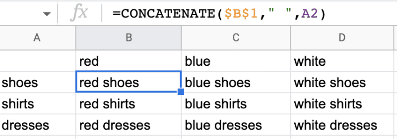
=CONCATENATE(A1,A2,A3)
CONCATENATE (documentation)
- =CONCATENATE(A1,A2,A3) you have the option to concatenate columns
- =CONCATENATE(A1,” I’m additional text”) or literal words and characters
Concatenate is one of the most commonly used Google Sheet formulas in SEO, and for good reason.
It can serve a variety of use cases, including creating keyword lists (concatenating two+ variables together), creating URL strings, or even bulk templatizing metadata.
As the name suggests, you can use it to simply string any amount of values together.
Just remember: if you need a space between keywords, a literal space “ “ must be added.
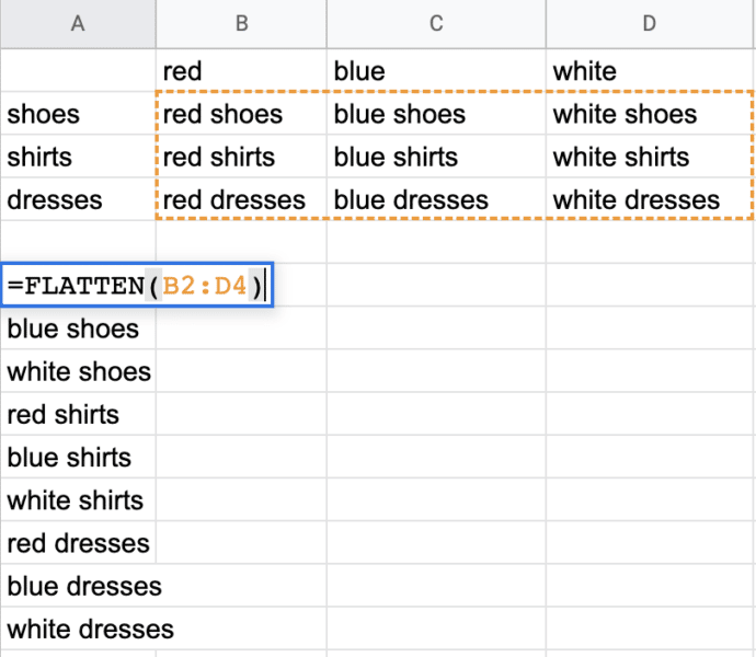
=FLATTEN(range1, [range2, …])
FLATTEN (documentation)
- =FLATTEN(A:D) would compress all ranges in A – D in to one column
There’s a reason FLATTEN is coming after concatenate. After you’ve concatenated several thousands of keywords and a couple of hundred dollars away, you generally need to upload the keywords into your rank tracking tool’s UI or via a CSV bulk upload.
It can be tedious when you have a 20×20 block of keywords to get them into a single column so you can upload all your keywords in one go.
With FLATTEN, you essentially select the range of data you want and the output is all of your keywords in one column to make copy-pasting a dream!
=LOWER(text)
LOWER (documentation)
This one’s pretty simple – but it can be helpful to LOWERcase all the of the keywords you’re managing (especially if you use a service provider that charges for things like duplicates) or if you’re in a case-sensitive environment like SQL.
LOWER is admittedly one of the simplest Google Sheets formulas for SEO.
The opposite (UPPER) also works, should you feel like auto-capping everything.

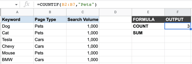
=COUNTIF(range,”[text or function]”)
COUNTIF (documentation)
COUNTIF lets you count, with accuracy, any literal text you want to match or even some numerical values that meet conditional rules.
It’s particularly useful when grouping together pages, managing an upcoming content calendar or sorting keywords on common dimensions like the page type or product they support.
It can also be used with conditions to match values, such as ones that have CPCs > $10.00 or that have a search volume > 100 searches a month.
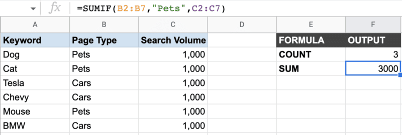
=SUMIF([range to search],”[condition to match]”,[range to return])
SUMIF (documentation)
SUMIF is similar to COUNTIF, but is helpful if you’re trying to add up an additional metric associated with the group of interest, like summing up total keyword volume opportunities by themes or search volume by page type.
Google Sheets formulas for internationalization
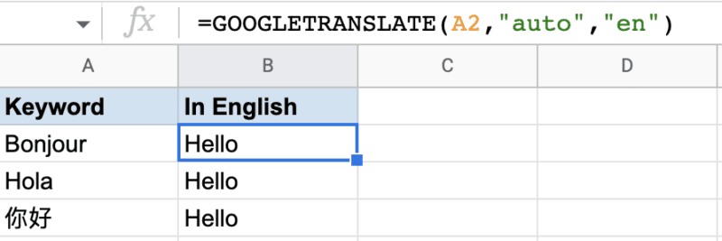
=GOOGLETRANSLATE(text, [“source_language” or “auto”, “target_language”])
GOOGLE TRANSLATE (documentation)
- source_language = two-letter language code of the source language (or “auto” for Google to guess)
- target_language = two-letter* language code for your target language, like ES for Spanish
Ahh, one of my favorite and most loved Google Sheets hacks.
Rather than go back and forth to the Google Translate UI and risk carpal tunnel, you can bulk translate lists of keywords in seconds into one, or even multiple languages.
You even have the option to auto-select the origin language by changing source_language to “auto” to let G sheets choose for you (which usually works, usually).
Google doesn’t support translating into all “flavors” of languages (e.g., Canadian French), but supports languages like pt-pt and pt-br, as well as Chinese languages like zh-tw and zh-cn.
Google Sheets formulas for content/URL management
=SPLIT(text,[delimiter wrapped in “”])
SPLIT (documentation)
Many times when you’re doing an analysis you might be working with data that is not in the required format you need.
There might be extraneous information that is separated (delimited) by things like commas (addresses), phone numbers (parenthesis and hyphens) and more.
While there’s a “split text to columns function” in the toolbar under “Data”, you can also split text that is delimited by a specific character, word or even spaces to individual columns with the SPLIT command directly in the sheet so you can quickly trim and tidy your keyword list.

=LEN(text)
LEN (documentation)
LEN is a simple Google Sheets formula for SEO you can use to simply count the characters in a line or string.
It can be most helpful when guiding people (both SEOs and non-SEOs) who are writing their own metadata, to stay within a “safe” enough character count so that it will hopefully not get truncated simply due to length.

=REGEXREPLACE(text, “regular_expression”, “replacement”)
REGEXREPLACE (documentation)
Regexes are a powerful data mining tool when working on large websites.
If you’ve never even heard of regexes, you’ve probably not yet been challenged with an enterprise-level site.
I find myself using REGEXREPLACE most often when I’m cleaning up or trimming URLs in a sheet, where it can be helpful when I only need a path name minus domain or to manage redirects.

Google Sheets formula for dashboards
=SPARKLINE(B3:G3)
SPARKLINE (documentation)
- =SPARKLINE(B3:G3,{“charttype”,”line”; “color”,”indigo”; “linewidth”,2}) this version of sparkline is in indigo, with a slightly heavier weight
While BI tools like Tableau and Looker offer additional customizations, Google Sheets can be a cheap way to build simple dashboards.
The command SPARKLINE is capable of leveraging data to create simple visualizations in a Google Sheet.
A good amount of SEO and web data looks great on a time series, and Google Sheets can make it easy.
This is most helpful when you have data that is being actively updated inside of Google Sheets and need to skim 10+ trends quickly in one sheet.
A popular use case is to monitor trends like growth in several countries, campaigns or city-level basis.
=SPARKLINE(B3:G3,{“charttype”,”line”; “color”,”[color you want]”; “linewidth”,2})
Time series/line charts
Time series is probably the most helpful for visualizing changes to traffic patterns over time and is suitable for monitoring most traffic trends and north star goals.
You can also remove the “line width” command, weight and even color for a quick and easy graph, but I find for time series I always need the line to be a little bolder and the contrasting color helps draw attention to the graph.

Column charts and bar charts
Sparkline even supports column and bar charts! Just change the chart type to column (shown below) or bar.

In more advanced use cases, most of the formulas above can be manipulated to have enhanced outputs, like automated conditional formatting or fun Unicode emoticon responses instead of nulls.
No matter how advanced you make them, using these formulas inside of Google Sheets is a great and cheap way to do basic SEO tidying work and keyword research.
The post 11 Google Sheets formulas SEOs should know appeared first on Search Engine Land.
from Search Engine Land https://ift.tt/Mi6oclE
via
No comments:
Post a Comment